
Stability Evaluation Approach
Stability studies support two key objectives. The first establishes an appropriate shelf life or retest period. The second evaluates whether product quality stays consistent during commercial manufacture and storage. Our approach addresses both objectives using established statistical methods aligned with international regulatory guidance.
1.Shelf-Life Estimation
Shelf life estimation follows the framework described in ICH Q1E Evaluation of Stability Data and ICH Q1A(R2) Stability Testing of New Drug Substances and Products.
The statistical foundation for this approach originates from the stability analysis procedure implemented in the FDA SAS STAB macro introduced in 1984. This method established a structured way to estimate expiry or retest intervals using regression analysis of stability data and has been widely adopted in regulatory submissions.
Subsequent regulatory guidance, including FDA stability guidance issued in 2004 and the ICH Q1E guideline published in 2003, follows the same statistical principles while allowing flexibility in how the models are applied. As a result, the analytical concepts introduced in the SAS STAB macro continue to underpin modern regulatory stability assessments.
-
Subsequent regulatory guidance, including FDA stability guidance issued in 2004 and the ICH Q1E guideline published in 2003, follows the same statistical principles while allowing flexibility in how the models are applied. As a result, the analytical concepts introduced in the SAS STAB macro continue to underpin modern regulatory stability assessments.
The approach uses an Analysis of Covariance (ANCOVA) model to evaluate how a quality attribute changes during storage while accounting for potential differences between manufacturing batches.Two variables are considered.
Time, representing the stability timepoint
Batch, representing the manufacturing lot
The model evaluates three components.
The overall change in the attribute with time
Differences between batches
Whether batches change at different rates over time
The analysis begins with a full model that allows each batch to have its own slope and intercept. This step determines whether the degradation rate differs between batches.
If the interaction between batch and time is not meaningful, the model simplifies by assuming that batches share a common slope while allowing each batch to have its own intercept.
If batch differences are also small, the data combine into a single pooled regression model with a common slope and intercept.
This hierarchical approach follows the statistical decision framework described in ICH Q1E, where a significance level of 0.25 is used when evaluating whether batch related effects should remain in the model. The relatively high threshold reflects a conservative strategy designed to avoid pooling batches that might behave differently.
Once the appropriate model has been selected, the regression trend describes how the stability attribute changes with time. Shelf life is estimated from the point where the confidence bound of the regression line intersects the relevant specification limit.
If batches behave differently, the most conservative batch determines the expiry estimate. If batches behave consistently, the pooled model provides a more precise estimate because it uses information from all available data.
This method provides a statistically justified estimate of the time when the product attribute could approach the specification boundary and forms the basis of regulatory shelf-life determination.
2.Lifecycle Stability Evaluation
(part of Continued/Ongoing Process Verification & Product Quality/Annual Product Review)
While regression analysis establishes labelled shelf life, stability data also provide valuable insight into product performance during the commercial lifecycle. Our evaluations therefore also apply structured data review to assess batch-to-batch behavior across stability timepoints.
Control charts provide a clear summary of stability performance across batches and support early identification of unusual variation or emerging trends. This lifecycle perspective aligns with the principles described in ICH Q10 Pharmaceutical Quality System and the direction of the emerging ICH Q1 Stability Guideline.
By combining regression modelling for shelf life estimation with lifecycle monitoring of stability behavior, this approach provides both regulatory compliance and deeper understanding of product stability performance.
i. Holistic Stability Model
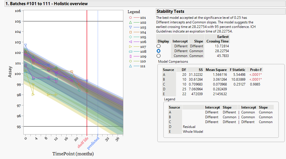
This figure shows the full stability dataset from eleven manufacturing batches. The registered shelf life for the product is twenty-four months.
Shelf-life evaluation follows the statistical framework described in ICH Q1A(R2) Stability Testing of New Drug Substances and Products and ICH Q1E Evaluation of Stability Data. The analysis uses a regression-based Analysis of Covariance (ANCOVA) model to evaluate how assay changes with storage time while considering differences between batches.
The model selected for this dataset allows different intercepts with a common slope. This means batches may start at slightly different assay levels, while the rate of degradation across time is assumed to be the same.
-
This model selection follows the hierarchical testing approach described in ICH Q1E. The analysis begins with the full model where both slope and intercept may differ between batches. Statistical testing then determines whether slope differences are significant. In this dataset, slope differences are not significant, so a common degradation rate is applied across all batches while retaining separate starting levels.
Using this model, the earliest projected crossing time of the specification limit occurs at approximately 28.2 months. Because the registered shelf life is 24 months,
the dataset supports the labelled shelf life under the ICH stability evaluation framework.At this stage the statistical requirement for shelf-life justification is satisfied. However, the model result also indicates that batches do not begin at identical assay levels. This observation becomes important when the dataset is reviewed from a lifecycle and batch-trending perspective, which is explored in the following analysis.
ii. Added Value of Process Behavior Chart
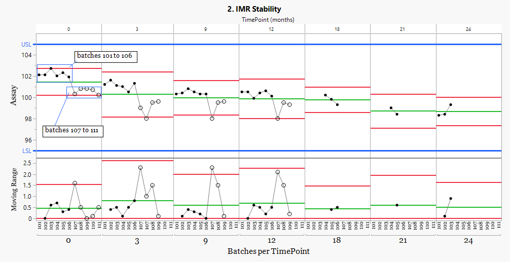
The process behavior chart shows that the dataset does not represent a single batch population. A clear step change occurs between batches 106 and 107, creating two stability populations.
While the pooled ANCOVA model supports the registered 24-month shelf life under the ICH stability framework, the control chart shows that batches from two manufacturing periods behave differently.
-
To understand the practical impact of this shift, the stability model can be applied separately to each population. This allows the degradation behavior of the earlier and later batches to be evaluated independently.
When the two groups are modelled separately, the difference becomes clear. The earlier batches show a much longer projected stability profile, while the later batches approach the specification limit much sooner.
Population-based modelling therefore reveals the practical impact of the batch shift and provides a clearer understanding of stability behavior across the manufacturing timeline.
iii. Population-Based Stability Modelling
Population 1 – Batches 101–106
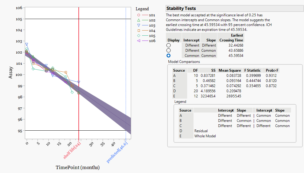
This figure shows the stability behavior of the earlier manufacturing population consisting of batches 101 to 106.
When these batches are evaluated independently, the statistical model again selects a common slope and common intercept structure. This indicates that both the starting assay levels and the degradation behavior across time are consistent within this batch group.
-
The projected stability model estimates the earliest specification crossing at approximately 45.5 months. This result is substantially longer than the registered shelf life of 24 months and confirms that this batch population demonstrates a stable and predictable degradation profile.
Within this group, the regression model and the underlying data show good alignment, with no indication of unusual batch behavior or divergence between stability timepoints.
This analysis confirms that the earlier manufacturing population provides a strong stability profile that comfortably supports the labelled shelf life.
Population 2 – Batches 107–111

This figure shows the stability behavior of the later manufacturing population consisting of batches 107 to 111.
When the stability model is applied to this group independently, the projected earliest crossing time occurs at approximately 23.6 months. This result sits close to the registered shelf life of 24 months and therefore represents the more limiting stability population within the dataset.
-
Although the degradation rate remains similar to the earlier batches, the starting assay levels are lower and the overall stability trajectory approaches the specification limit more rapidly.
This result explains the intercept difference detected in the pooled ANCOVA stability model and confirms that the two batch populations behave differently across the stability timeline.
The population-based analysis therefore reveals the practical impact of the batch shift. While the pooled stability model supports the labelled shelf life statistically, the later manufacturing population represents the controlling stability behavior for the product.
iv. Conclusions
Regression modelling establishes shelf life in line with ICH stability guidance and supports regulatory submissions. Process behavior charts add another layer of understanding by revealing how the data evolve across the manufacturing timeline. Used together, these approaches allow stability data to be interpreted both statistically and operationally.
-
In this example the statistical model alone supports the registered shelf life. The process behavior chart reveals a clear step change linked to a manufacturing site transition. This additional perspective highlights a shift in batch population behavior which would otherwise remain hidden inside the pooled model.
Verto Pharma therefore applies both stability modelling and process behavior analysis as standard practice. Stability models provide the regulatory estimate. Process behavior charts provide visibility of manufacturing performance and change over time.
A common misconception suggests that process behavior charts require 20 to 25 observations before useful insight emerges. In practice, meaningful signals often appear much earlier. Even with four to five batches, stability data can already show whether a product behaves as a single population or whether shifts between manufacturing periods require closer investigation.
This combined approach strengthens stability assessment, improves detection of manufacturing changes, and supports a more robust understanding of product performance throughout the commercial lifecycle.